
An example of drawing up a variational series. Solution: I
Depending on the trait underlying the formation of a distribution series, there are attribute and variation distribution series.
The presence of a common feature is the basis for the formation of a statistical population, which is the results of a description or measurement of common features of the objects of study.
The subject of study in statistics are changing (varying) features or statistical features.
Types of statistical features.
Distribution series are called attribute series. built on quality grounds. Attributive- this is a sign that has a name (for example, a profession: a seamstress, teacher, etc.).
It is customary to arrange the distribution series in the form of tables. In table. 2.8 shows an attribute series of distribution.
Table 2.8 - Distribution of types of legal assistance provided by lawyers to citizens of one of the regions of the Russian Federation.
Variation series are distribution series built on a quantitative basis. Any variational series consists of two elements: variants and frequencies.
Variants are individual values of a feature that it takes in a variation series.
Frequencies are the numbers of individual variants or each group variation series, i.e. these are numbers showing how often certain options occur in a distribution series. The sum of all frequencies determines the size of the entire population, its volume.
Frequencies are called frequencies, expressed in fractions of a unit or as a percentage of the total. Accordingly, the sum of the frequencies is equal to 1 or 100%. The variational series allows us to evaluate the form of the distribution law based on actual data.
Depending on the nature of the variation of the trait, there are discrete and interval variation series.
An example of a discrete variational series is given in Table. 2.9.
Table 2.9 - Distribution of families by the number of rooms occupied in individual apartments in 1989 in the Russian Federation.
Variation series
In the general population, a certain quantitative trait is being investigated. A sample of volume is randomly extracted from it n, that is, the number of elements in the sample is n. At the first stage of statistical processing, ranging samples, i.e. number ordering x 1 , x 2 , …, x n Ascending. Each observed value x i called option. Frequency m i is the number of observations of the value x i in the sample. Relative frequency (frequency) w i is the frequency ratio m i to sample size n: .When studying a variational series, the concepts of cumulative frequency and cumulative frequency are also used. Let x some number. Then the number of options , whose values are less x, is called the accumulated frequency: for x i
An attribute is called discretely variable if its individual values (variants) differ from each other by some finite amount (usually an integer). A variational series of such a feature is called a discrete variational series.
Table 1. General view of the discrete variational series of frequencies
| Feature values | x i | x 1 | x2 | … | x n |
| Frequencies | m i | m 1 | m2 | … | m n |
An attribute is called continuously varying if its values differ from each other by an arbitrarily small amount, i.e. the sign can take any value in a certain interval. A continuous variation series for such a trait is called an interval series.
Table 2. General view of the interval variation series of frequencies
Table 3. Graphic images of the variation series
| Row | Polygon or histogram | Empirical distribution function | |
| Discrete | 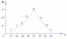 |  |  |
| interval |  | 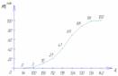 | 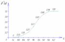 |
For graphic representation of variational series, polygon, histogram, cumulative curve and empirical distribution function are most often used.
In table. 2.3 (Grouping of the population of Russia according to the size of the average per capita income in April 1994) is presented interval variation series.
It is convenient to analyze the distribution series using a graphical representation, which also makes it possible to judge the shape of the distribution. A visual representation of the nature of the change in the frequencies of the variational series is given by polygon and histogram.
The polygon is used when displaying discrete variational series.
Let us depict, for example, graphically the distribution of housing stock by type of apartments (Table 2.10).
Table 2.10 - Distribution of the housing stock of the urban area by type of apartments (conditional figures).

Rice. Housing distribution polygon
On the y-axis, not only the values of frequencies, but also the frequencies of the variation series can be plotted.
The histogram is taken to display the interval variation series. When constructing a histogram, the values of the intervals are plotted on the abscissa axis, and the frequencies are depicted by rectangles built on the corresponding intervals. The height of the columns in the case of equal intervals should be proportional to the frequencies. A histogram is a graph in which a series is shown as bars adjacent to each other.
Let's graphically depict the interval distribution series given in Table. 2.11.
Table 2.11 - Distribution of families by the size of living space per person (conditional figures).
| N p / p | Groups of families by the size of living space per person | Number of families with a given size of living space | Accumulated number of families |
| 1 | 3 – 5 | 10 | 10 |
| 2 | 5 – 7 | 20 | 30 |
| 3 | 7 – 9 | 40 | 70 |
| 4 | 9 – 11 | 30 | 100 |
| 5 | 11 – 13 | 15 | 115 |
| TOTAL | 115 | ---- | |

Rice. 2.2. Histogram of the distribution of families by the size of living space per person
Using the data of the accumulated series (Table 2.11), we construct distribution cumulative.

Rice. 2.3. The cumulative distribution of families by the size of living space per person
The representation of a variational series in the form of a cumulate is especially effective for variational series, the frequencies of which are expressed as fractions or percentages of the sum of the frequencies of the series.
If we change the axes in the graphic representation of the variational series in the form of a cumulate, then we get ogivu. On fig. 2.4 shows an ogive built on the basis of the data in Table. 2.11.
A histogram can be converted to a distribution polygon by finding the midpoints of the sides of the rectangles and then connecting these points with straight lines. The resulting distribution polygon is shown in fig. 2.2 dotted line.
When constructing a histogram of the distribution of a variational series with unequal intervals, along the ordinate axis, not frequencies are applied, but the distribution density of the feature in the corresponding intervals.
The distribution density is the frequency calculated per unit interval width, i.e. how many units in each group are per unit interval value. An example of calculating the distribution density is presented in Table. 2.12.
Table 2.12 - Distribution of enterprises by the number of employees (figures are conditional)
| N p / p | Groups of enterprises by the number of employees, pers. | Number of enterprises | Interval size, pers. | Distribution density |
| BUT | 1 | 2 | 3=1/2 | |
| 1 | up to 20 | 15 | 20 | 0,75 |
| 2 | 20 – 80 | 27 | 60 | 0,25 |
| 3 | 80 – 150 | 35 | 70 | 0,5 |
| 4 | 150 – 300 | 60 | 150 | 0,4 |
| 5 | 300 – 500 | 10 | 200 | 0,05 |
| TOTAL | 147 | ---- | ---- |
For a graphical representation of variation series can also be used cumulative curve. With the help of the cumulate (the curve of the sums), a series of accumulated frequencies is displayed. Accumulated frequencies are determined by sequentially summing the frequencies by groups and show how many units of the population have feature values no greater than the considered value.

Rice. 2.4. Ogiva distribution of families according to the size of living space per person
When constructing the cumulate of an interval variation series, the variants of the series are plotted along the abscissa axis, and the accumulated frequencies along the ordinate axis.
Continuous variation series
A continuous variational series is a series built on the basis of a quantitative statistical sign. Example. The average duration of diseases of convicts (days per person) in the autumn-winter period in the current year was:| 7,0 | 6,0 | 5,9 | 9,4 | 6,5 | 7,3 | 7,6 | 9,3 | 5,8 | 7,2 |
| 7,1 | 8,3 | 7,5 | 6,8 | 7,1 | 9,2 | 6,1 | 8,5 | 7,4 | 7,8 |
| 10,2 | 9,4 | 8,8 | 8,3 | 7,9 | 9,2 | 8,9 | 9,0 | 8,7 | 8,5 |
Glossary of statistical terms
General questions of statistics
WHAT IS MEDICAL STATISTICS?
Statistics is a quantitative description and measurement of events, phenomena, objects. It is understood as a branch of practical activity (collection, processing and analysis of data on mass phenomena), as a branch of knowledge, i.e. a special scientific discipline, and as a set of summary, final digital indicators collected to characterize any area of social phenomena.
Statistics is a science that studies the patterns of mass phenomena by the method of generalizing indicators.
Medical statistics is an independent social science that studies the quantitative side of mass social phenomena inextricably linked with their qualitative side, allowing generalizing indicators method to study the patterns of these phenomena, the most important processes in the economic and social life of society, its health, and the system of organizing medical care for the population.
Statistical methods are a set of techniques for processing materials of mass observations, which include: grouping, summary, obtaining indicators, their statistical analysis, etc.
Statistical methods in medicine are used to:
- studying the state of public health of the population as a whole and its main groups by collecting and analyzing statistical data on the size and composition of the population, its reproduction, physical development, prevalence and duration of various diseases, etc.;
- identification and establishment of links between the general level of morbidity and mortality from any individual diseases with various environmental factors;
- collection and study of numerical data on the network of medical institutions, their activities and personnel for planning health care activities, monitoring the implementation of plans for the development of the network and activities of health institutions and assessing the quality of work of individual medical institutions;
- assessment of the effectiveness of measures to prevent and treat diseases;
- determination of the statistical significance of the results of the study in the clinic and experiment.
Sections of medical statistics:
- general theoretical and methodological foundations of statistics,
- population health statistics,
- health statistics.
CREATING A DATABASE IN MS EXCEL
In order for the database to be convenient for further processing, simple principles should be followed:
1) The best program for creating a database is MS Excel. Data from Excel can later be easily transferred to other specialized statistical packages, such as Statistica, SPSS, etc. for more complex manipulations. However, up to 80-90% of the calculations can be most conveniently performed in Excel itself using the Data Analysis add-in.
2) The top line of the table with the database is designed as a header, where the names of those indicators that are taken into account in this column are entered. It is undesirable to use cell merging (this requirement applies to the entire database in general), since in this case many operations will become invalid. Also, you should not create a "two-story" header, in which the top line indicates the name of a group of homogeneous indicators, and the bottom line - specific indicators. To group homogeneous indicators, it is better to mark them with a single-color fill or include a grouping feature in brackets in their name.
For example, not this way:
| GENERAL BLOOD ANALYSIS | ||
| ER | LEU | TR |
| ER(UAC) | LEU(UAC) | TR(UAC) |
in the latter version, both the “one-story” header and the visual homogeneity of the data are ensured (all of them refer to the UAC indicators).
3) The first column should contain the serial number of the patient in this database, without linking it to any of the studied indicators. This will make it possible in the future to provide an easy rollback to the original order of patients at any stage, even after numerous sortings of the list.
4) The second column is usually filled with the names (or full names) of the patients.
5) Quantitative indicators (those that are measured by numbers, for example - height, weight, blood pressure, heart rate, etc.) fit into the table in a numerical format. It would seem that this is already clear, but it should be remembered that in Excel, starting from the 2007 version, fractional values are denoted by a dot: 4.5. If you write a number separated by a comma, then it will be perceived as text, and these columns will have to be rewritten.
6) With qualitative indicators it is more difficult. Those that have two meanings (the so-called binary values: Yes-No, Available-Absent, Male-Female), it is better to translate into a binary system: 0 and 1. The value 1 is usually assigned to a positive value (Yes, Available) , 0 - negative (No, None).
7) Qualitative indicators that have several values that differ in severity, the level of the phenomenon (Weak-Medium-Strong; Cold-Warm-Hot) can be ranked and, accordingly, also translated into numbers. The lowest level of the phenomenon is assigned the lowest rank - 0 or 1, the next degrees are indicated by the values of the ranks in order. For example: No disease - 0, mild - 1, moderate - 2, severe - 3.
8) Sometimes one quality indicator corresponds to several values. For example, in the "Concomitant diagnosis" column, if there are several diseases, we want to indicate them separated by commas. This should not be done, since the processing of such data is very difficult and cannot be automated. Therefore, it is better to make several columns with specific groups of diseases ("CVD diseases", "diseases of the gastrointestinal tract", etc.) or certain nosologies ("chr.gastritis", "IHD", etc.), in which the data is entered into binary, binary form: 1 (which means "There is a given disease") - 0 ("There is no given disease").
9) To distinguish between individual groups of indicators, you can actively use color: for example, columns with KLA indicators are highlighted in red, OAM data - in yellow, etc.
10) Each patient should correspond to one line of the table.
Such a design of the database allows not only to significantly simplify the process of its statistical processing, but also to facilitate its filling at the stage of collecting material.
WHICH METHOD TO CHOOSE FOR STATISTICAL ANALYSIS?
After collecting all the data, each researcher faces the question of choosing the most appropriate method of statistical processing. And this is not surprising: modern statistics combines a huge number of various criteria and methods. All of them have their own characteristics, may or may not be suitable for two seemingly similar situations. In this article, we will try to systematize all the main, most common methods of statistical analysis according to their purpose.
However, first, a few words about what kind of statistical data there are, since the choice of the most appropriate method of analysis depends on this.
Measurement scale
When conducting a study, the values of various features are determined for each unit of observation. Depending on the scale on which they are measured, all signs are divided into quantitative and quality. Qualitative indicators in research are distributed according to the so-called nominal scale. In addition, indicators can be presented by ranking scale.
For example, a comparison is made of indicators of cardiac activity in athletes and persons leading a sedentary lifestyle.
At the same time, the following characteristics were determined in the subjects:
- floor- is nominal an indicator that takes two values - male or female.
- age - quantitative index,
- sports - nominal an indicator that takes two values: engaged or not engaged,
- heart rate - quantitative index,
- systolic blood pressure - quantitative index,
- complaints of chest pain- is quality indicator, the values of which can be determined as nominal(there are complaints - there are no complaints), and according to ranking a scale depending on the frequency (for example, if the pain occurs several times a day - the indicator is assigned a rank of 3, several times a month - a rank of 2, several times a year - a rank of 1, if there are no complaints of chest pain - a rank of 0 is assigned) .
Number of matched populations
The next issue that needs to be addressed in order to select a statistical method is the number of populations to be matched within the study.
- In most cases, in clinical trials, we deal with two groups of patients - basic and control. Basic, or experienced, is considered to be the group in which the studied method of diagnosis or treatment was used, or in which patients suffer from the disease that is the subject of this study. control the group, in contrast, consists of patients receiving conventional medical care, placebo, or individuals who do not have the disease under study. Such populations represented by different patients are called unrelated.
There are still related, or paired, aggregates, when it comes to the same people, but the values of any feature are compared, obtained before and after research. The number of compared sets is also equal to 2, but different methods are applied to them than to unrelated ones. - Another option is description one totality, which, admittedly, underlies any research in general. Even if the main purpose of the work is to compare two or more groups, each of them must first be characterized. For this, methods are used descriptive statistics. In addition, for a single population, methods can be applied correlation analysis, used to find a relationship between two or more of the characteristics under study (for example, the dependence of height on body weight or the dependence of heart rate on body temperature).
- Finally, there can be several compared sets. This is very common in medical research. Patients can be grouped depending on the use of various drugs (for example, when comparing the effectiveness of antihypertensive drugs: group 1 - ACE inhibitors, 2 - beta-blockers, 3 - centrally acting drugs), according to the severity of the disease (group 1 - mild, 2 - medium, 3 - heavy), etc.
Also important is the question distribution normality studied populations. It depends on whether methods can be applied parametric analysis or only nonparametric. The conditions that must be met in normally distributed populations are:
- maximum proximity or equality of the values of the arithmetic mean, mode and median;
- compliance with the "three sigma" rule (at least 68.3% of the variant is in the interval M ± 1σ, at least 95.5% of the variant is in the interval of M ± 2σ, at least 99.7% of the variant is in the interval of M ± 3σ;
- indicators are measured in a quantitative scale;
- positive results of testing for the normality of distribution using special criteria - Kolmogorov-Smirnov or Shapiro-Wilk.
After determining all the characteristics of the studied populations indicated by us, we suggest using the following table to select the most optimal method of statistical analysis.
| Method | Scale for measuring indicators | Number of compared populations | Purpose of processing | Data distribution |
| Student's t-test | quantitative | 2 | normal | |
| Student's t-test with Bonferroni correction | quantitative | 3 or more | comparison of unrelated populations | normal |
| Paired Student's t-test | quantitative | 2 | normal | |
| One-way analysis of variance (ANOVA) | quantitative | 3 or more | comparison of unrelated populations | normal |
| One-way analysis of variance (ANOVA) with repeated measures | quantitative | 3 or more | comparison of related populations | normal |
| Mann-Whitney U test | quantitative, ranking | 2 | comparison of unrelated populations | any |
| Rosenbaum Q-test | quantitative, ranking | 2 | comparison of unrelated populations | any |
| Kruskell-Wallis test | quantitative | 3 or more | comparison of unrelated populations | any |
| Wilcoxon test | quantitative, ranking | 2 | comparison of related populations | any |
| G-test signs | quantitative, ranking | 2 | comparison of related populations | any |
| Friedman criterion | quantitative, ranking | 3 or more | comparison of related populations | any |
| Criterion χ 2 Pearson | nominal | 2 or more | comparison of unrelated populations | any |
| Fisher's exact test | nominal | 2 | comparison of unrelated populations | any |
| McNemar test | nominal | 2 | comparison of related populations | any |
| Q-test Cochran | nominal | 3 or more | comparison of related populations | any |
| Relative risk (Risk Ratio, RR) | nominal | 2 | comparison of unrelated populations in cohort studies | any |
| Odds Ratio (OR) | nominal | 2 | comparison of unrelated populations in case-control studies | any |
| Pearson correlation coefficient | quantitative | 2 rows of measurements | normal | |
| Spearman's rank correlation coefficient | quantitative, ranking | 2 rows of measurements | identifying relationships between features | any |
| Kendall's correlation coefficient | quantitative, ranking | 2 rows of measurements | identifying relationships between features | any |
| Kendall's Concordance Coefficient | quantitative, ranking | 3 or more rows of measurements | identifying relationships between features | any |
| Calculation of mean values (M) and mean errors (m) | quantitative | 1 | descriptive statistics | any |
| Calculation of medians (Me) and percentiles (quartiles) | ranking | 1 | descriptive statistics | any |
| Calculation of relative values (P) and average errors (m) | nominal | 1 | descriptive statistics | any |
| Shapiro-Wilk criterion | quantitative | 1 | distribution analysis | any |
| Kolmogorov-Smirnov criterion | quantitative | 1 | distribution analysis | any |
| Criterion ω 2 Smirnov-Kramer-von Mises | quantitative | 1 | distribution analysis | any |
| Kaplan-Meier method | any | 1 | survival analysis | any |
| Cox proportional hazards model | any | 1 | survival analysis | any |
Great statisticians
Karl Pearson (March 27, 1857 - April 27, 1936)
March 27, 1857 was born Karl Pearson - the great English mathematician, statistician, biologist and philosopher; founder of mathematical statistics, one of the founders of biometrics.
After receiving a professorship in applied mathematics at University College London at the age of 27, Karl Pearson began to study statistics, which he perceived as a general scientific tool, consistent with his far from conventional ideas about the need to provide students with a broad outlook.
Pearson's main achievements in the field of statistics include the development of the foundations of the theory of correlation and contingency of features, the introduction of "Pearson curves" to describe empirical distributions and the extremely important chi-square test, and the compilation of a large number of statistical tables. Pearson applied the statistical method and especially the theory of correlation in many branches of science.
Here is one of his statements: "The first amateur introduction of modern statistical methods into established science is opposed by typical contempt. But I lived to the time when many of them began to covertly apply the very methods that they initially condemned."
And already in 1920, Pearson wrote a note in which he stated that the goal of the biometric school was "to transform statistics into a branch of applied mathematics, to generalize, discard or justify the meager methods of the old school of political and social statisticians, and, in general, to transform statistics from the sports ground for amateurs and debaters into a serious branch of science. It was necessary to criticize the imperfect and often erroneous methods in medicine, anthropology, craniometry, psychology, criminology, biology, sociology, in order to provide these sciences with new and more powerful means. The battle lasted almost twenty years, but many signs that the old hostility is behind us and the new methods are universally accepted.
Karl Pearson had very versatile interests: he studied physics in Heidelberg, was interested in the social and economic role of religion, and even lectured on German history and literature in Cambridge and London.
It is a little-known fact that at the age of 28, Karl Pearson lectured on the "women's question" and even founded the Men's and Women's Club, which existed until 1889, in which everything related to women, including relations between the sexes, was freely and unrestrictedly discussed.
The club consisted of an equal number of men and women, mostly liberal middle class, socialists and feminists.
The subject of the club's discussions was the widest range of issues: from sexual relations in ancient Greek Athens to the position of Buddhist nuns, from attitudes towards marriage to prostitution problems. In essence, the "Club of men and women" challenged long-established norms of interaction between men and women, as well as ideas about the "correct" sexuality. In Victorian England, where many perceived sexuality as something “low” and “animal”, and ignorance about sex education was widespread, the discussion of such issues was really radical.
In 1898, Pearson was awarded the Royal Society's Darwin Medal, which he refused, believing that awards "should be given to young people to encourage them."
Florence Nightingale (May 12, 1820 - August 13, 1910)
Florence Nightingale (1820-1910) - sister of mercy and public figure of Great Britain, on whose birthday we celebrate International Nurse's Day today.
She was born in Florence in a wealthy aristocratic family, received an excellent education, knew six languages. From a young age she dreamed of becoming a sister of mercy, in 1853 she received a nursing education in the community of the sisters of Pastor Flender in Kaiserwerth and became the manager of a small private hospital in London.
In October 1854, during the Crimean War, Florence, along with 38 assistants, went to field hospitals in the Crimea. Organizing the care of the wounded, she consistently implemented the principles of sanitation and hygiene. As a result, in less than six months, the death rate in hospitals decreased from 42 to 2.2%!
Setting herself the task of reforming the medical service in the army, Nightingale ensured that hospitals were equipped with ventilation and sewage systems; Hospital staff must have received the necessary training. A military medical school was organized, and explanatory work was carried out among soldiers and officers on the importance of disease prevention.
Florence Nightingale's contribution to medical statistics is great!
- Her 800-page book, Notes on the Factors Influencing the Health, Efficiency, and Administration of the Hospitals of the British Army (1858), contained an entire section devoted to statistics and illustrated with diagrams.
- Nightingale was an innovator in the use of graphic images in statistics. She invented pie charts, which she called "cockscombs" and used to describe patterns of mortality. Many of her diagrams were included in the report of the commission on health problems in the army, thanks to which the decision was made to reform army medicine.
- She developed the first form for collecting statistics in hospitals, which is the forerunner of modern reporting forms on the activities of the hospital.
In 1859 she was elected a Fellow of the Royal Statistical Society and subsequently became an honorary member of the American Statistical Association.
⠀Johann Carl Friedrich Gauss (April 30, 1777 - February 23, 1855)
On April 30, 1777, the great German mathematician, mechanic, physicist, astronomer, surveyor and statistician Johann Carl Friedrich Gauss was born in Braunschweig.
He is considered one of the greatest mathematicians of all time, the "King of Mathematicians". Laureate of the Copley medal (1838), foreign member of the Swedish (1821) and Russian (1824) Academies of Sciences, of the English Royal Society.
Already at the age of three, Karl could read and write, even correcting his father's counting errors. According to legend, a school mathematics teacher, in order to keep children busy for a long time, invited them to count the sum of numbers from 1 to 100. Young Gauss noticed that pairwise sums from opposite ends are the same: 1+100=101, 2+99=101, etc. etc., and instantly got the result: 50×101=5050. Until old age, he used to do most of the calculations in his mind.
The main scientific achievements of Carl Gauss in statistics are the creation of the least squares method, which underlies regression analysis.
He also studied in detail the normal distribution law common in nature, the graph of which has since often been called the Gaussian. The three-sigma rule (Gaussian rule) describing the normal distribution has become widely known.
Lev Semyonovich Kaminsky (1889 - 1962)
On the 75th anniversary of the Victory in the Great Patriotic War, I would like to remember and talk about the remarkable scientist, one of the founders of military medical and sanitary statistics in the USSR - Lev Semyonovich Kaminsky (1889-1962).
He was born on May 27, 1889 in Kyiv. After graduating with honors in 1918 from the medical faculty of Petrograd University, Kaminsky was in the ranks of the Red Army, from April 1919 until the end of 1920 he served as chief physician of the 136th consolidated evacuation hospital of the South-Eastern Front.
Since 1922, Lev Semyonovich was in charge of the sanitary and epidemiological department of the medical and sanitary service of the North-Western Railway. During these years, the scientific activity of Kaminsky began under the guidance of prof. S.A.Novoselsky. In their joint fundamental work “Losses in Past Wars”, statistical material was analyzed on human losses in the wars of various armies of the world from 1756 to 1918. In subsequent works, Kaminsky developed and substantiated a new, more accurate classification of military losses.
In the monograph "National nutrition and public health" (1929), the sanitary and hygienic aspects of the impact of wars on the health of the population, as well as the organization of medical care for the population and the army during the war years, were considered in detail.
From 1935 to 1943, Lev Semenovich headed the department of sanitary (since 1942 - medical) statistics of the People's Commissariat of Health of the USSR. In October 1943, Prof. Kaminsky became the head of the Department of Military Medical Statistics of the Military Medical Academy. S.M. Kirov, and since 1956 he has been a professor at the Department of Statistics and Accounting at the Leningrad State University.
Lev Semyonovich advocated the widespread introduction of quantitative methods into the practice of sanitary and medical statistics. In 1959, under his authorship, a textbook "Statistical processing of laboratory and clinical data: the use of statistics in the scientific and practical work of a doctor" was published, which for many years became one of the best domestic textbooks on medical statistics. In the preface, L.S. Kaminsky notes:
"... It seems important that the attending physicians know how to get down to business, be able to collect and process the correct numbers, suitable for comparisons and comparisons."
Criteria and methods
Student's t-test for independent populations
Student's t-test is a general name for a class of methods for statistical testing of hypotheses (statistical tests) based on the Student's distribution. The most common cases of applying the t-test are related to checking the equality of the means in two samples.
This criterion was developed William Seeley Gosset
2. What is the Student's t-test used for?
Student's t-test is used to determine the statistical significance of mean differences. It can be used both in cases of comparison of independent samples (for example, groups of patients with diabetes mellitus and groups of healthy people), and when comparing related populations (for example, the average pulse rate in the same patients before and after taking an antiarrhythmic drug). In the latter case, the paired Student's t-test is calculated
3. When can the Student's t-test be used?
To apply the Student's t-test, it is necessary that the original data have a normal distribution. Also important is the equality of dispersions (distributions) of the compared groups (homoscedasticity). For unequal variances, the Welch's t-test is used (Welch "s t).
In the absence of a normal distribution of the compared samples, instead of the Student's t-test, similar methods of nonparametric statistics are used, among which the most famous is Mann-Whitney U-test.
4. How to calculate Student's t-test?
To compare means, Student's t-test is calculated using the following formula:
where M 1- arithmetic mean of the first compared population (group), M 2- arithmetic mean of the second compared population (group), m 1- the average error of the first arithmetic mean, m2- the average error of the second arithmetic mean.
The resulting value of Student's t-test must be correctly interpreted. To do this, we need to know the number of subjects in each group (n 1 and n 2). Finding the number of degrees of freedom f according to the following formula:
F \u003d (n 1 + n 2) - 2
After that, we determine the critical value of Student's t-test for the required level of significance (for example, p=0.05) and for a given number of degrees of freedom f according to the table (see below).
- If the calculated value of the Student's t-test is equal to or greater than the critical value found in the table, we conclude that the differences between the compared values are statistically significant.
- If the value of the calculated Student's t-test is less than the tabular one, then the differences between the compared values are not statistically significant.
To study the effectiveness of a new iron preparation, two groups of patients with anemia were selected. In the first group, patients received a new drug for two weeks, and in the second group they received a placebo. After that, the level of hemoglobin in peripheral blood was measured. In the first group, the average hemoglobin level was 115.4±1.2 g/l, and in the second - 103.7±2.3 g/l (data are presented in M±m format), the compared populations have a normal distribution. The number of the first group was 34, and the second - 40 patients. It is necessary to draw a conclusion about the statistical significance of the obtained differences and the effectiveness of the new iron preparation.
Solution: To assess the significance of differences, we use Student's t-test, calculated as the difference between the means divided by the sum of squared errors:
After performing the calculations, the value of the t-test was equal to 4.51. We find the number of degrees of freedom as (34 + 40) - 2 = 72. We compare the obtained value of Student's t-test 4.51 with the critical value at p=0.05 indicated in the table: 1.993. Since the calculated value of the criterion is greater than the critical value, we conclude that the observed differences are statistically significant (significance level p<0,05).
PAIRED STUDENT'S t-test
Paired Student's t-test is one of the modifications of Student's method used to determine the statistical significance of differences in paired (repeated) measurements.
1. History of the development of the t-test
t-test was developed William Gosset to assess the quality of beer at Guinness. In connection with obligations to the company not to disclose trade secrets, Gosset's article was published in 1908 in the journal Biometrics under the pseudonym "Student" (Student).
2. What is the paired Student's t-test used for?
Paired Student's t-test is used to compare two dependent (paired) samples. Dependent are measurements taken in the same patients but at different times, for example, blood pressure in hypertensive patients before and after taking an antihypertensive drug. The null hypothesis states that there are no differences between the compared samples, while the alternative hypothesis states that there are statistically significant differences.
3. When can paired Student's t-test be used?
The main condition is the dependence of the samples, that is, the compared values should be obtained by repeated measurements of one parameter in the same patients.
As in the case of comparing independent samples, in order to apply the paired t-test, it is necessary that the original data have a normal distribution. If this condition is not met, non-parametric statistics methods, such as G-test signs or Wilcoxon t-test.
The paired t-test can only be used when comparing two samples. If you want to compare three or more repeated measurements, you should use one-way analysis of variance (ANOVA) for repeated measures.
4. How to calculate paired Student's t-test?
The paired Student's t-test is calculated using the following formula:
where M d- the arithmetic mean of the differences between the indicators measured before and after, σd- standard deviation of the differences of indicators, n- the number of subjects.
5. How to interpret the value of Student's t-test?
The interpretation of the obtained value of the paired Student's t-test does not differ from the evaluation of the t-test for unrelated populations. First of all, it is necessary to find the number of degrees of freedom f according to the following formula:
F = n - 1
After that, we determine the critical value of Student's t-test for the required significance level (for example, p<0,05) и при данном числе степеней свободы f according to the table (see below).
We compare the critical and calculated values of the criterion:
- If the calculated value of the paired Student's t-test is equal to or greater than the critical value found in the table, we conclude that the differences between the compared values are statistically significant.
- If the value of the calculated paired Student's t-test is less than the table value, then the differences between the compared values are not statistically significant.
6. An example of calculating the Student's t-test
To evaluate the effectiveness of a new hypoglycemic agent, blood glucose levels were measured in patients with diabetes mellitus before and after taking the drug. As a result, the following data were obtained:
Solution:
1. Calculate the difference of each pair of values (d):
| Patient N | Blood glucose level, mmol/l | Value difference (d) | |
| before taking the drug | after taking the drug | ||
| 1 | 9.6 | 5.7 | 3.9 |
| 2 | 8.1 | 5.4 | 2.7 |
| 3 | 8.8 | 6.4 | 2.4 |
| 4 | 7.9 | 5.5 | 2.4 |
| 5 | 9.2 | 5.3 | 3.9 |
| 6 | 8.0 | 5.2 | 2.8 |
| 7 | 8.4 | 5.1 | 3.3 |
| 8 | 10.1 | 6.9 | 3.2 |
| 9 | 7.8 | 7.5 | 2.3 |
| 10 | 8.1 | 5.0 | 3.1 |
2. Find the arithmetic mean of the differences using the formula:
3. Find the standard deviation of the differences from the average by the formula:
4. Calculate the paired Student's t-test:
5. Let's compare the obtained value of Student's t-test 8.6 with the tabular value, which, with the number of degrees of freedom f equal to 10 - 1 = 9 and the significance level p=0.05, is 2.262. Since the obtained value is greater than the critical one, we conclude that there are statistically significant differences in blood glucose levels before and after taking the new drug.
MANN-WHITNEY U-CRITERION
The Mann-Whitney U-test is a non-parametric statistical test used to compare two independent samples in terms of the level of any trait, measured quantitatively. The method is based on determining whether the area of intersecting values between two variational series is sufficiently small (a ranged series of parameter values in the first sample and the same in the second sample). The smaller the criterion value, the more likely it is that the differences between the parameter values in the samples are significant.
1. History of the development of the U-test
This method for detecting differences between samples was proposed in 1945 by an American chemist and statistician Frank Wilcoxon.
In 1947, it was substantially revised and expanded by mathematicians H.B. Mann(H.B. Mann) and D.R. Whitney(D.R. Whitney), by whose names it is usually called today.
2. What is the Mann-Whitney U-test used for?
The Mann-Whitney U-test is used to assess the differences between two independent samples in terms of the level of any quantitative trait.
3. When can the Mann-Whitney U test be used?
The Mann-Whitney U-test is a non-parametric test, therefore, unlike Student's t-test
The U-test is suitable for comparing small samples: each sample must contain at least 3 feature values. It is allowed that in one sample there are 2 values, but in the second one then there must be at least five.
The condition for applying the Mann-Whitney U-test is the absence in the compared groups of coinciding attribute values (all numbers are different) or a very small number of such matches.
An analogue of the Mann-Whitney U-test for comparing three or more groups is Kruskal-Wallis test.
4. How to calculate the Mann-Whitney U-test?
First, from both compared samples, single ranked row, by arranging the units of observation according to the degree of increase of the attribute and assigning a lower value to a lower rank. In the case of equal attribute values for several units, each of them is assigned the arithmetic mean of successive rank values.
For example, two units that occupy 2nd and 3rd place (rank) in a single ranked row have the same values. Therefore, each of them is assigned a rank equal to (3 + 2) / 2 = 2.5.
In the compiled single ranked series, the total number of ranks will be equal to:
N = n 1 + n 2
where n 1 is the number of elements in the first sample and n 2 is the number of elements in the second sample.
Next, we again divide the single ranked series into two, consisting, respectively, of the units of the first and second samples, while remembering the values of the ranks for each unit. We calculate separately the sum of the ranks that fell on the share of the elements of the first sample, and separately - on the share of the elements of the second sample. Determine the larger of the two rank sums (T x) corresponding to the sample with n x elements.
Finally, we find the value of the Mann-Whitney U-test using the formula:
5. How to interpret the value of the Mann-Whitney U-test?
The obtained value of the U-criterion is compared according to the table for the chosen level of statistical significance (p=0.05 or p=0.01) with the critical value of U for a given number of compared samples:
- If the resulting value U less tabular or equals to him, then the statistical significance of the differences between the levels of the trait in the considered samples is recognized (an alternative hypothesis is accepted). The significance of differences is higher, the lower the value of U.
- If the resulting value U more tabular, the null hypothesis is accepted.
WILCOXON CRITERION
Wilcoxon's test for linked samples (also known as Wilcoxon's T-test, Wilcoxon's test, Wilcoxon's signed rank test, Wilcoxon's rank sum test) is a non-parametric statistical test used to compare two linked (paired) samples by the level of any quantitative trait measured on a continuous or ordinal scale.
The essence of the method is that the absolute values of the severity of shifts in one direction or another are compared. To do this, first all the absolute values of the shifts are ranked, and then the ranks are summed up. If shifts in one direction or another happen by chance, then the sums of their ranks will be approximately equal. If the intensity of shifts in one direction is greater, then the sum of the ranks of the absolute values of shifts in the opposite direction will be significantly lower than it could be with random changes.
1. History of the development of the Wilcoxon test for linked samples
The test was first proposed in 1945 by American statistician and chemist Frank Wilcoxon (1892-1965). In the same scientific work, the author described another criterion used in the case of comparing independent samples.
2. What is the Wilcoxon test used for?
The Wilcoxon t-test is used to evaluate the differences between two sets of measurements performed on the same population of subjects, but under different conditions or at different times. This test is able to reveal the direction and severity of changes - that is, whether the indicators are more shifted in one direction than in the other.
A classic example of a situation in which the Wilcoxon T-test for related populations can be applied is a before-after study, where pre- and post-treatment scores are compared. For example, when studying the effectiveness of an antihypertensive agent, blood pressure is compared before taking the drug and after taking it.
3. Conditions and restrictions on the use of the Wilcoxon T-test
- The Wilcoxon test is a non-parametric test, therefore, unlike paired Student's t-test, does not require the presence of a normal distribution of the compared populations.
- The number of subjects when using the Wilcoxon T-test must be at least 5.
- The trait under study can be measured both on a quantitative continuous scale (blood pressure, heart rate, leukocyte count per 1 ml of blood) and on an ordinal scale (number of points, severity of the disease, degree of contamination by microorganisms).
- This criterion is used only when comparing two series of measurements. An analogue of the Wilcoxon T-test for comparing three or more related populations is Friedman criterion.
4. How to calculate the Wilcoxon T-test for related samples?
- Calculate the difference between the values of paired measurements for each subject. Zero shifts are not taken into account further.
- Determine which of the differences are typical, that is, they correspond to the direction of change of the indicator prevailing in frequency.
- Rank the differences of the pairs by their absolute values (that is, without taking into account the sign), in ascending order. A lower absolute value of the difference is assigned a lower rank.
- Calculate the sum of ranks corresponding to atypical shifts.
Thus, the Wilcoxon T-test for related samples is calculated by the following formula:
where ΣRr is the sum of ranks corresponding to atypical changes in the indicator.
5. How to interpret the value of the Wilcoxon test?
The obtained value of the Wilcoxon T-test is compared with the critical value according to the table for the selected level of statistical significance ( p=0.05 or p=0.01) for a given number of compared samples n:
- If the calculated (empirical) value of Temp. less than the tabular T cr. or equal to it, then the statistical significance of changes in the indicator in the typical direction is recognized (an alternative hypothesis is accepted). The significance of differences is higher, the lower the value of T.
- If Temp. more T cr. , the null hypothesis about the absence of statistical significance of the indicator changes is accepted.
An example of calculating the Wilcoxon test for related samples
A pharmaceutical company is conducting research on a new drug from the group of non-steroidal anti-inflammatory drugs. For this, a group of 10 volunteers suffering from acute respiratory viral infections with hyperthermia was selected. Their body temperature was measured before and 30 minutes after taking the new drug. It is required to draw a conclusion about the significance of the decrease in body temperature as a result of taking the drug.
- The initial data are presented in the form of the following table:
- To calculate the Wilcoxon T-test, we calculate the differences in paired indicators and rank their absolute values. At the same time, atypical ranks will be highlighted in red:
As we see typical shift indicator is its decrease, noted in 7 cases out of 10. In one case (in patient Egorov), the temperature did not change after taking the drug, and therefore this case was not used in further analysis. In two cases (in patients of Sidorov and Alekseev) atypical shift temperature upwards. The ranks corresponding to the atypical shift are 1.5 and 3.N Surname t of the body before taking the drug t of the body after taking the drug Difference of indicators, d |d| Rank 1. Ivanov 39.0 37.6 -1.4 1.4 7 2. Petrov 39.5 38.7 -0.8 0.8 5 3. Sidorov 38.6 38.7 0.1 0.1 1.5 4. Popov 39.1 38.5 -0.6 0.6 4 5. Nikolaev 40.1 38.6 -1.5 1.5 8 6. Kozlov 39.3 37.5 -1.8 1.8 9 7. Ignatiev 38.9 38.8 -0.1 0.1 1.5 8. Semenov 39.2 38.0 -1.2 1.2 6 9. Egorov 39.8 39.8 0 — — 10. Alekseev 38.8 39.3 0.5 0.5 3 - We calculate the Wilcoxon T-test, which is equal to the sum of the ranks corresponding to the atypical shift of the indicator:
T = ΣRr = 3 + 1.5 = 4.5
- Compare Temp. with T cr. , which at the significance level p=0.05 and n=9 is equal to 8. Therefore, T emp.
- We conclude that the decrease in body temperature in patients with ARVI as a result of taking a new drug is statistically significant (p<0.05).
PEARSON'S CHI-SQUARE test
The Pearson χ2 test is a non-parametric method that allows you to evaluate the significance of differences between the actual (revealed as a result of the study) number of outcomes or qualitative characteristics of the sample that fall into each category and the theoretical number that can be expected in the studied groups if the null hypothesis is true. In simpler terms, the method allows you to evaluate the statistical significance of differences between two or more relative indicators (frequencies, shares).
1. History of the development of the χ 2 criterion
The chi-square test for the analysis of contingency tables was developed and proposed in 1900 by an English mathematician, statistician, biologist and philosopher, the founder of mathematical statistics and one of the founders of biometrics Karl Pearson(1857-1936).
2. What is Pearson's χ 2 criterion used for?
The chi-square test can be applied in the analysis contingency tables containing information about the frequency of outcomes depending on the presence of a risk factor. For example, a four-field contingency table looks like this:
| Exodus is (1) | No exit (0) | Total | |
| There is a risk factor (1) | A | B | A+B |
| No risk factor (0) | C | D | C+D |
| Total | A+C | B+D | A+B+C+D |
How to fill in such a contingency table? Let's consider a small example.
A study is underway on the effect of smoking on the risk of developing arterial hypertension. For this, two groups of subjects were selected - the first included 70 people who smoke at least 1 pack of cigarettes daily, the second - 80 non-smokers of the same age. In the first group, 40 people had high blood pressure. In the second - arterial hypertension was observed in 32 people. Accordingly, normal blood pressure in the group of smokers was in 30 people (70 - 40 = 30) and in the group of non-smokers - in 48 (80 - 32 = 48).
We fill in the four-field contingency table with the initial data:
In the resulting contingency table, each line corresponds to a specific group of subjects. Columns - show the number of persons with arterial hypertension or with normal blood pressure.
The challenge for the researcher is: are there statistically significant differences between the frequency of people with blood pressure among smokers and non-smokers? You can answer this question by calculating Pearson's chi-square test and comparing the resulting value with the critical one.
- Comparable indicators should be measured on a nominal scale (for example, the patient's gender - male or female) or in an ordinal scale (for example, the degree of arterial hypertension, which takes values from 0 to 3).
- This method allows analysis not only of four-field tables, when both the factor and the outcome are binary variables, that is, they have only two possible values (for example, male or female, the presence or absence of a certain disease in history ...). Pearson's chi-square test can also be used in the case of the analysis of multi-field tables, when the factor and (or) outcome take three or more values.
- The matched groups should be independent, i.e. the chi-square test should not be used when comparing before-after observations. McNemar test(when comparing two related populations) or calculated Q-test Cochran(in case of comparing three or more groups).
- When analyzing four-field tables expected values in each of the cells must be at least 10. In the event that in at least one cell the expected phenomenon takes a value from 5 to 9, the chi-square test must be calculated with Yates correction. If in at least one cell the expected phenomenon is less than 5, then the analysis should use Fisher's exact test.
- In the case of analysis of multi-field tables, the expected number of observations should not take values less than 5 in more than 20% of the cells.
4. How to calculate Pearson's chi-square test?
To calculate the chi-square test, you must:
This algorithm is applicable for both four-field and multi-field tables.
5. How to interpret the value of Pearson's chi-square test?
In the event that the obtained value of the criterion χ 2 is greater than the critical one, we conclude that there is a statistical relationship between the studied risk factor and the outcome at the appropriate level of significance.
6. An example of calculating the Pearson chi-square test
Let us determine the statistical significance of the influence of the smoking factor on the incidence of arterial hypertension according to the table above:
- We calculate the expected values for each cell:
- Find the value of Pearson's chi-square test:
χ 2 \u003d (40-33.6) 2 / 33.6 + (30-36.4) 2 / 36.4 + (32-38.4) 2 / 38.4 + (48-41.6) 2 / 41.6 \u003d 4.396.
- The number of degrees of freedom f = (2-1)*(2-1) = 1. We find the critical value of the Pearson chi-square test from the table, which, at a significance level of p=0.05 and the number of degrees of freedom 1, is 3.841.
- We compare the obtained value of the chi-square test with the critical one: 4.396 > 3.841, therefore, the dependence of the incidence of arterial hypertension on the presence of smoking is statistically significant. The significance level of this relationship corresponds to p<0.05.
FISHER'S EXACT CRITERION
Fisher's exact test is a test that is used to compare two relative indicators that characterize the frequency of a particular trait that has two values. The initial data for calculating Fisher's exact test are usually grouped in the form of a four-field table.
1. History of the development of the criterion
The criterion was first proposed Ronald Fisher in his book Design of Experiments. This happened in 1935. Fisher himself claimed that Muriel Bristol prompted this idea. In the early 1920s, Ronald, Muriel and William Roach were in England at an experimental agricultural station. Muriel claimed to be able to determine the sequence in which tea and milk were poured into her cup. At that time, it was not possible to verify the correctness of her statement.
This gave rise to Fisher's idea of the "null hypothesis". The goal was not to try to prove that Muriel could tell the difference between differently prepared cups of tea. It was decided to refute the hypothesis that a woman makes a choice at random. It was determined that the null hypothesis can neither be proven nor substantiated. But it can be refuted during experiments.
8 cups were made. In the first four, milk is poured first, in the other four - tea. The cups were messed up. Bristol was invited to taste the tea and divide the cups according to the method of making tea. The result should have been two groups. History says that the experiment was a success.
Thanks to the Fisher test, the probability that Bristol is acting intuitively has been reduced to 0.01428. That is, it was possible to correctly determine the cup in one case out of 70. But still, there is no way to reduce to zero the chances that Madame determines by chance. Even if you increase the number of cups.
This story gave impetus to the development of the "null hypothesis". At the same time, Fisher's exact test was proposed, the essence of which is to enumerate all possible combinations of dependent and independent variables.
2. What is Fisher's exact test used for?
Fisher's exact test is mainly used to compare small samples. There are two significant reasons for this. First, the calculation of the criterion is rather cumbersome and can take a lot of time or require powerful computing resources. Secondly, the criterion is quite accurate (which is reflected even in its name), which allows it to be used in studies with a small number of observations.
A special place is given to Fisher's exact criterion in medicine. This is an important method of processing medical data, which has found its application in many scientific studies. Thanks to it, it is possible to investigate the relationship of certain factors and outcomes, to compare the frequency of pathological conditions between two groups of subjects, etc.
3. In what cases can Fisher's exact test be used?
- Comparable variables should be measured on a nominal scale and have only two values, for example, blood pressure is normal or elevated, the outcome is favorable or unfavorable, there are postoperative complications or not.
- Fisher's exact test is designed to compare two independent groups divided by factor. Accordingly, the factor must also have only two possible values.
- The test is suitable for comparing very small samples: Fisher's exact test can be used to analyze four-complete tables in case of expected phenomena values less than 5, which is a limitation for application Pearson's chi-square test, even with the Yates correction.
- Fisher's exact test can be unilateral or bilateral. With a one-sided option, it is known exactly where one of the indicators will deviate. For example, a study compares how many patients recovered compared to a control group. It is assumed that therapy cannot worsen the condition of patients, but only either cure or not.
The two-tailed test evaluates frequency differences in two directions. That is, the probability of both a higher and a lower frequency of the phenomenon in the experimental group compared to the control group is estimated.
An analogue of Fisher's exact test is Pearson's chi-square test, while Fisher's exact test has a higher power, especially when comparing small samples, and therefore has an advantage in this case.
4. How to calculate Fisher's exact test?
For example, we study the dependence of the frequency of birth of children with congenital malformations (CMD) on maternal smoking during pregnancy. For this, two groups of pregnant women were selected, one of which is experimental, consisting of 80 women who smoked in the first trimester of pregnancy, and the second is a comparison group, including 90 women leading a healthy lifestyle throughout pregnancy. The number of cases of fetal CM in the experimental group was 10, in the comparison group - 2.
First, we compile a four-field contingency table:
Fisher's exact test is calculated using the following formula:
where N is the total number of subjects in the two groups; ! - factorial, which is the product of a number and a sequence of numbers, each of which is less than the previous one by 1 (for example, 4! = 4 3 2 1)
As a result of calculations, we find that P = 0.0137.
5. How to interpret the value of Fisher's exact test?
The advantage of the method is the correspondence of the obtained criterion to the exact value of the significance level p. That is, the value of 0.0137 obtained in our example is the level of significance of the differences between the compared groups in terms of the incidence of fetal CM. It is only necessary to compare this number with the critical level of significance, usually taken in medical research as 0.05.
- If the value of Fisher's exact test is greater than the critical one, the null hypothesis is accepted and a conclusion is made that there are no statistically significant differences in the frequency of outcome depending on the presence of a risk factor.
- If the value of Fisher's exact test is less than the critical one, an alternative hypothesis is accepted and a conclusion is made about the presence of statistically significant differences in the frequency of outcome depending on the impact of the risk factor.
In our example P< 0,05, в связи с чем делаем вывод о наличии прямой взаимосвязи курения и вероятности развития ВПР плода. Частота возникновения врожденной патологии у детей курящих женщин статистически значимо выше, чем у некурящих.
Odds ratio
The odds ratio is a statistical indicator (in Russian its name is usually abbreviated as OSH, and in English - OR from "odds ratio"), one of the main ways to describe in numerical terms how much the absence or presence of a certain outcome is associated with the presence or absence of a certain factor in a specific statistical group.
1. History of the development of the odds ratio indicator
The term "chance" came from the theory of gambling, where with the help of this concept they denoted the ratio of winning positions to losing ones. In the scientific medical literature, the odds ratio indicator was first mentioned in 1951 in the work of J. Kornfield. Subsequently, this researcher published papers that noted the need to calculate a 95% confidence interval for the odds ratio. (Cornfield, J. A Method for Estimating Comparative Rates from Clinical Data. Applications to Cancer of the Lung, Breast, and Cervix // Journal of the National Cancer Institute, 1951. - N.11. - P.1269–1275.)
2. What is the odds ratio used for?
The odds ratio allows you to evaluate the relationship between a certain outcome and a risk factor.
The odds ratio allows you to compare groups of subjects in terms of the frequency of identifying a particular risk factor. It is important that the result of applying the odds ratio is not only the determination of the statistical significance of the relationship between the factor and the outcome, but also its quantitative assessment.
3. Conditions and restrictions on the application of the odds ratio
- Performance and factor indicators should be measured on a nominal scale. For example, the resultant sign is the presence or absence of a congenital malformation in the fetus, the studied factor is the mother's smoking (smoking or not smoking).
- This method allows the analysis of only four-field tables, when both the factor and the outcome are binary variables, that is, they have only two possible values (for example, gender - male or female, arterial hypertension - presence or absence, outcome of the disease - with or without improvement ...).
- Matched groups should be independent, that is, the odds ratio is not suitable for comparing before-after observations.
- The odds ratio indicator is used in case-control studies (for example, the first group - patients with hypertension, the second - relatively healthy people). For prospective studies, when groups are formed on the basis of the presence or absence of a risk factor (for example, the first group - smokers, the second group - non-smokers), can also be calculated relative risk.
4. How to calculate the odds ratio?
The odds ratio is the value of the fraction, in the numerator of which are the chances of a certain event for the first group, and in the denominator are the chances of the same event for the second group.
chance is the ratio of the number of subjects who have a certain feature (outcome or factor) to the number of subjects who do not have this feature.
For example, a group of patients operated on for pancreatic necrosis was selected, the number of which was 100 people. After 5 years, 80 of them survived. Accordingly, the chance of survival was 80 to 20, or 4.
A convenient way is to calculate the odds ratio with data summarized in a 2x2 table:
| Exodus is (1) | No exit (0) | Total | |
| There is a risk factor (1) | A | B | A+B |
| No risk factor (0) | C | D | C+D |
| Total | A+C | B+D | A+B+C+D |
For this table, the odds ratio is calculated using the following formula:
It is very important to evaluate the statistical significance of the identified relationship between the outcome and the risk factor. This is due to the fact that even with low values of the odds ratio close to one, the relationship, nevertheless, may turn out to be significant and should be taken into account in statistical conclusions. Conversely, at large OR values, the indicator turns out to be statistically insignificant, and, therefore, the revealed relationship can be neglected.
To assess the significance of the odds ratio, the boundaries of the 95% confidence interval are calculated (the abbreviation 95% CI or 95% CI from the English "confidence interval" is used). The formula for finding the value of the upper limit of 95% CI:
The formula for finding the value of the lower limit of 95% CI:
5. How to interpret the value of the odds ratio?
- If the odds ratio is greater than 1, then this means that the chances of finding a risk factor are greater in the group with an outcome. Those. factor has a direct relationship with the likelihood of an outcome.
- An odds ratio less than 1 indicates that the chances of finding a risk factor are greater in the second group. Those. factor has an inverse relationship with the probability of the outcome.
- With an odds ratio equal to one, the chances of finding a risk factor in the compared groups are the same. Accordingly, the factor has no effect on the probability of the outcome.
Additionally, in each case, the statistical significance of the odds ratio is necessarily assessed based on the values of the 95% confidence interval.
- If the confidence interval does not include 1, i.e. both values of the limits are either above or below 1, a conclusion is made about the statistical significance of the identified relationship between the factor and the outcome at a significance level of p<0,05.
- If the confidence interval includes 1, i.e. its upper limit is greater than 1, and the lower limit is less than 1, it is concluded that there is no statistical significance of the relationship between the factor and the outcome at a significance level of p>0.05.
- The value of the confidence interval is inversely proportional to the level of significance of the relationship between the factor and the outcome, i.e. the smaller the 95% CI, the more significant the identified relationship.
6. An example of calculating the odds ratio indicator
Imagine two groups: the first consisted of 200 women who were diagnosed with a congenital malformation of the fetus (Outcome+). Of these, smoked during pregnancy (Factor+) - 50 people (BUT), were non-smokers (Factor-) - 150 people (FROM).
The second group consisted of 100 women without signs of fetal malformations (Outcome -), among whom 10 people smoked during pregnancy (Factor +) (B), did not smoke (Factor-) - 90 people (D).
1. Compile a four-field contingency table:
2. Calculate the value of the odds ratio:
OR = (A * D) / (B * C) = (50 * 90) / (150 * 10) = 3.
3. Find the boundaries of 95% CI. The value of the lower limit calculated according to the above formula was 1.45, and the upper limit was 6.21.
Thus, the study showed that the chances of meeting a smoking woman among patients diagnosed with fetal CM are 3 times higher than among women without signs of fetal CM. The observed dependence is statistically significant, since 95% of CI does not include 1, the values of its lower and upper limits are greater than 1.
RELATIVE RISK
Risk is the likelihood of a particular outcome, such as illness or injury. The risk can take values from 0 (there is no probability of an outcome) to 1 (an unfavorable outcome is expected in all cases). In medical statistics, as a rule, changes in the risk of an outcome depending on some factor are studied. Patients are conditionally divided into 2 groups, one of which is affected by the factor, the other is not.
Relative risk is the ratio of the frequency of outcomes among subjects affected by the factor under study to the frequency of outcomes among subjects not affected by that factor. In the scientific literature, the abbreviated name of the indicator is often used - RR or RR (from the English "relative risk").
1. History of the development of the relative risk indicator
The calculation of relative risk is borrowed by medical statistics from economics. A correct assessment of the influence of political, economic and social factors on the demand for a product or service can lead to success, and an underestimation of these factors can lead to financial failures and bankruptcy of the enterprise.
2. What is relative risk used for?
Relative risk is used to compare the likelihood of an outcome depending on the presence of a risk factor. For example, when assessing the effect of smoking on the incidence of hypertension, when studying the dependence of the incidence of breast cancer on oral contraceptives, etc. Relative risk is the most important indicator in prescribing certain treatments or conducting studies with possible side effects.
3. Conditions and restrictions on the use of relative risk
- Factor and outcome measures should be measured on a nominal scale (eg, patient gender, male or female, hypertension present or not).
- This method allows analysis of only four-field tables when both the factor and the outcome are inary variables, that is, they have only two possible values (for example, age under or over 50 years, the presence or absence of a specific disease in history).
- Relative risk is used in prospective studies, when study groups are formed on the basis of the presence or absence of a risk factor. In case-control studies, the relative risk should be replaced by the indicator odds ratio.
4. How to calculate relative risk?
To calculate the relative risk, it is necessary:
5. How to interpret the relative risk value?
The relative risk score is compared with 1 in order to determine the nature of the relationship between the factor and the outcome:
- If the RR is 1, it can be concluded that the factor under study does not affect the probability of the outcome (no relationship between the factor and the outcome).
- At values greater than 1, it is concluded that the factor increases the frequency of outcomes (direct relationship).
- At values less than 1 - about a decrease in the probability of an outcome under the influence of a factor (feedback).
The values of the boundaries of the 95% confidence interval are also necessarily estimated. If both values - both the lower and upper limits - are on the same side of 1, or, in other words, the confidence interval does not include 1, then a conclusion is made about the statistical significance of the identified relationship between the factor and the outcome with the probability of error p<0,05.
If the lower limit of the 95% CI is less than 1, and the upper limit is greater, then it is concluded that there is no statistical significance of the influence of the factor on the outcome rate, regardless of the RR value (p>0.05).
6. An example of calculating the relative risk indicator
In 1999, studies were conducted in Oklahoma on the incidence of men with stomach ulcers. Regular consumption of fast food was chosen as an influencing factor. In the first group there were 500 men who constantly eat fast food, among which stomach ulcers were diagnosed in 96 people. The second group included 500 supporters of a healthy diet, among whom a stomach ulcer was diagnosed in 31 cases. Based on the data obtained, the following contingency table was built:
PEARSON CORRELATION CRITERION
Pearson's correlation test is a parametric statistics method that allows you to determine the presence or absence of a linear relationship between two quantitative indicators, as well as evaluate its closeness and statistical significance. In other words, the Pearson correlation test allows you to determine whether one indicator changes (increases or decreases) in response to changes in another? In statistical calculations and inferences, the correlation coefficient is usually denoted as r xy or R xy .
1. History of the development of the correlation criterion
The Pearson correlation test was developed by a team of British scientists led by Karl Pearson(1857-1936) in the 90s of the 19th century, to simplify the analysis of the covariance of two random variables. In addition to Karl Pearson, Pearson's correlation test was also worked on Francis Edgeworth and Raphael Weldon.
2. What is Pearson's correlation test used for?
The Pearson correlation criterion allows you to determine what is the closeness (or strength) of the correlation between two indicators measured on a quantitative scale. With the help of additional calculations, you can also determine how statistically significant the identified relationship is.
For example, using the Pearson correlation criterion, one can answer the question of whether there is a relationship between body temperature and the content of leukocytes in the blood in acute respiratory infections, between the height and weight of the patient, between the content of fluoride in drinking water and the incidence of caries in the population.
3. Conditions and restrictions on the use of Pearson's chi-square test
- Comparable indicators should be measured on a quantitative scale (for example, heart rate, body temperature, leukocyte count per 1 ml of blood, systolic blood pressure).
- By means of the Pearson correlation criterion, it is possible to determine only the presence and strength of a linear relationship between the quantities. Other characteristics of the connection, including the direction (direct or reverse), the nature of the changes (straight or curvilinear), as well as the dependence of one variable on another, are determined using regression analysis.
- The number of values to be compared must be equal to two. In the case of analyzing the relationship of three or more parameters, you should use the method factor analysis.
- The Pearson correlation test is parametric, and therefore the condition for its application is the normal distribution of each of the compared variables. If it is necessary to perform a correlation analysis of indicators whose distribution differs from the normal one, including those measured on an ordinal scale, one should use Spearman's rank correlation coefficient.
- It is necessary to clearly distinguish between the concepts of dependence and correlation. The dependence of the values determines the presence of a correlation between them, but not vice versa.
For example, the growth of a child depends on his age, that is, the older the child, the taller he is. If we take two children of different ages, then with a high degree of probability the growth of the older child will be greater than that of the younger. This phenomenon is called dependence, implying a causal relationship between indicators. Of course, there is also a correlation between them, meaning that changes in one indicator are accompanied by changes in another indicator.
In another situation, consider the relationship between the growth of the child and the heart rate (HR). As you know, both of these values are directly dependent on age, therefore, in most cases, children of greater stature (and, therefore, older ones) will have lower heart rate values. That is, a correlation will be observed and may have a fairly high tightness. However, if we take children of the same age but different heights, then, most likely, their heart rate will differ insignificantly, and therefore we can conclude that heart rate is independent of growth.
This example shows how important it is to distinguish between the concepts of connection and dependence of indicators, which are fundamental in statistics, in order to draw correct conclusions.
4. How to calculate the Pearson correlation coefficient?
Pearson's correlation coefficient is calculated using the following formula:
5. How to interpret the value of the Pearson correlation coefficient?
The values of the Pearson correlation coefficient are interpreted based on its absolute values. Possible values of the correlation coefficient vary from 0 to ±1. The greater the absolute value of r xy, the higher the closeness of the relationship between the two quantities. r xy = 0 indicates a complete lack of connection. r xy = 1 - indicates the presence of an absolute (functional) connection. If the value of the Pearson correlation criterion turned out to be greater than 1 or less than -1, an error was made in the calculations.
To assess the closeness, or strength, of the correlation, generally accepted criteria are used, according to which the absolute values of r xy< 0.3 свидетельствуют о weak connection, r xy values from 0.3 to 0.7 - about connection middle tightness, r xy values > 0.7 - o strong connections.
A more accurate assessment of the strength of the correlation can be obtained using the Chaddock table:
The assessment of the statistical significance of the correlation coefficient r xy is carried out using a t-test calculated using the following formula:
The obtained value t r is compared with the critical value at a certain level of significance and the number of degrees of freedom n-2. If t r exceeds t crit, then a conclusion is made about the statistical significance of the identified correlation.
6. An example of calculating the Pearson correlation coefficient
The aim of the study was to identify, determine the tightness and statistical significance of the correlation between two quantitative indicators: the level of testosterone in the blood (X) and the percentage of muscle mass in the body (Y). The initial data for a sample consisting of 5 subjects (n = 5) are summarized in the table:
SPEERMAN'S CRITERION
Spearman's rank correlation coefficient is a non-parametric method that is used to statistically study the relationship between phenomena. In this case, the actual degree of parallelism between the two quantitative series of the studied features is determined and the tightness of the established relationship is estimated using a quantitatively expressed coefficient.
1. History of the development of the rank correlation coefficient
This criterion was developed and proposed for correlation analysis in 1904 Charles Edward Spearman, English psychologist, professor at London and Chesterfield Universities.
2. What is the Spearman ratio used for?
Spearman's rank correlation coefficient is used to identify and evaluate the closeness of the relationship between two series of compared quantitative indicators. In the event that the ranks of indicators, sorted by degree of increase or decrease, in most cases coincide (a higher value of one indicator corresponds to a higher value of another indicator - for example, when comparing a patient's height and his body weight), a conclusion is made about the presence straight correlation. If the ranks of indicators have the opposite direction (a higher value of one indicator corresponds to a lower value of the other - for example, when comparing age and heart rate), then they talk about reverse links between indicators.
- The Spearman correlation coefficient has the following properties:
- The correlation coefficient can take values from minus one to one, and at rs=1 there is a strictly direct relationship, and at rs= -1 - strictly inverse relationship.
- If the correlation coefficient is negative, then there is an inverse relationship; if it is positive, then there is a direct relationship.
- If the correlation coefficient is equal to zero, then the relationship between the quantities is practically absent.
- The closer the modulus of the correlation coefficient is to unity, the stronger is the relationship between the measured values.
3. In what cases can the Spearman coefficient be used?
Due to the fact that the coefficient is a method of non-parametric analysis, a check for the normality of the distribution is not required.
Comparable indicators can be measured both on a continuous scale (for example, the number of erythrocytes in 1 μl of blood) and on an ordinal scale (for example, peer review scores from 1 to 5).
The effectiveness and quality of Spearman's estimation is reduced if the difference between the different values of any of the measured quantities is large enough. It is not recommended to use the Spearman coefficient if there is an uneven distribution of the values of the measured value.
4. How to calculate Spearman's ratio?
The calculation of the Spearman rank correlation coefficient includes the following steps:
5. How to interpret the value of the Spearman coefficient?
When using the rank correlation coefficient, the closeness of the connection between the signs is conditionally estimated, considering the values of the coefficient less than 0.3 - a sign of weak closeness of the connection; values greater than 0.3 but less than 0.7 are a sign of moderate closeness of association, and values of 0.7 or more are a sign of high closeness of association.
Also, to assess the closeness of the connection, one can use Chaddock scale.
The statistical significance of the obtained coefficient is assessed using Student's t-test. If the calculated value of the t-criterion is less than the tabular value for a given number of degrees of freedom, the statistical significance of the observed relationship is absent. If more, then the correlation is considered statistically significant.
THE KOLMOGOROV-SMIRNOV METHOD
The Kolmogorov-Smirnov test is a non-parametric goodness-of-fit test, in the classical sense, designed to test simple hypotheses about the analyzed sample belonging to some known distribution law. The most well-known application of this criterion is to test the studied populations for normal distribution.
1. History of the development of the Kolmogorov-Smirnov criterion
The Kolmogorov-Smirnov criterion was developed by Soviet mathematicians Andrey Nikolaevich Kolmogorov and Nikolai Vasilyevich Smirnov.
Kolmogorov A.N. (1903-1987) - Hero of Socialist Labor, professor at Moscow State University, academician of the Academy of Sciences of the USSR - the greatest mathematician of the 20th century, is one of the founders of modern probability theory.
Smirnov N.V. (1900-1966) Corresponding member of the Academy of Sciences of the USSR, one of the founders of non-parametric methods of mathematical statistics and the theory of limit distributions of order statistics.
Subsequently, the Kolmogorov-Smirnov goodness-of-fit test was modified to be used to test populations for normal distribution by an American statistician, professor at George Washington University Hubert Lilliefors(Hubert Whitman Lilliefors, 1928-2008). Professor Lilliefors was one of the pioneers in the use of computer technology in statistical calculations.
Hubert Lilliefors2. What is the Kolmogorov-Smirnov criterion used for?
This criterion makes it possible to assess the significance of differences between the distributions of two samples, including its possible use to assess whether the distribution of the sample under study corresponds to the normal distribution law.
3. In what cases can the Kolmogorov-Smirnov criterion be used?
The Kolmogorov-Smirnov test is designed to test for the normality of the distribution of sets of quantitative data.
For greater reliability of the data obtained, the volumes of the considered samples should be large enough: n ≥ 50. With the size of the estimated population from 25 to 50 elements, it is advisable to use the Bolshev correction.
4. How to calculate the Kolmogorov-Smirnov criterion?
The Kolmogorov-Smirnov criterion is calculated using special statistical programs. It is based on statistics of the form:
where sup S is the least upper bound of the set S, F n- distribution function of the studied population, F(x)- normal distribution function
The inferred probability values are based on the assumption that the mean and standard deviation of the normal distribution are known a priori and are not estimated from the data.
However, in practice, the parameters are usually computed directly from the data. In this case, the normality test includes a complex hypothesis ("how likely is it to obtain a D statistic of given or greater significance, depending on the mean and standard deviation computed from the data"), and Lilliefors probabilities (Lilliefors, 1967) are given.
5. How to interpret the value of the Kolmogorov-Smirnov criterion?
If D the Kolmogorov-Smirnov statistic is significant (p<0,05), то гипотеза о том, что соответствующее распределение нормально, должна быть отвергнута.
A special place in statistical analysis belongs to the determination of the average level of the studied trait or phenomenon. The average level of a feature is measured by average values.
The average value characterizes the general quantitative level of the studied trait and is a group property of the statistical population. It levels, weakens the random deviations of individual observations in one direction or another and highlights the main, typical property of the trait under study.
Averages are widely used:
1. To assess the health status of the population: characteristics of physical development (height, weight, chest circumference, etc.), identifying the prevalence and duration of various diseases, analyzing demographic indicators (natural population movement, average life expectancy, population reproduction, average population and etc.).
2. To study the activities of medical institutions, medical personnel and assess the quality of their work, planning and determining the needs of the population in various types of medical care (average number of applications or visits per inhabitant per year, average length of stay of a patient in a hospital, average duration of examination patient, average provision with doctors, beds, etc.).
3. To characterize the sanitary and epidemiological state (average dustiness of the air in the workshop, average area per person, average consumption of proteins, fats and carbohydrates, etc.).
4. To determine the medical and physiological parameters in the norm and pathology, in the processing of laboratory data, to establish the reliability of the results of a selective study in socio-hygienic, clinical, experimental studies.
Calculation of average values is performed on the basis of variation series. Variation series- this is a qualitatively homogeneous statistical set, the individual units of which characterize the quantitative differences of the studied feature or phenomenon.
Quantitative variation can be of two types: discontinuous (discrete) and continuous.
A discontinuous (discrete) sign is expressed only as an integer and cannot have any intermediate values (for example, the number of visits, the population of the site, the number of children in the family, the severity of the disease in points, etc.).
A continuous sign can take on any values within certain limits, including fractional ones, and is expressed only approximately (for example, weight - for adults you can limit yourself to kilograms, and for newborns - grams; height, blood pressure, time spent on seeing a patient, and etc.).
The digital value of each individual feature or phenomenon included in the variation series is called a variant and is indicated by the letter V . There are also other notations in the mathematical literature, for example x or y.
A variational series, where each option is indicated once, is called simple. Such series are used in most statistical problems in the case of computer data processing.
With an increase in the number of observations, as a rule, there are repeated values of the variant. In this case, it creates grouped variation series, where the number of repetitions is indicated (frequency, denoted by the letter " R »).
Ranked variation series consists of options arranged in ascending or descending order. Both simple and grouped series can be composed with ranking.
Interval variation series are made up in order to simplify subsequent calculations performed without using a computer, with a very large number of observation units (more than 1000).
Continuous variation series includes variant values, which can be any value.
If in the variation series the values of the attribute (options) are given in the form of separate specific numbers, then such a series is called discrete.
The general characteristics of the values of the attribute reflected in the variation series are the average values. Among them, the most used are: the arithmetic mean M, fashion Mo and median me. Each of these characteristics is unique. They cannot replace each other, and only in the aggregate, quite fully and in a concise form, are the features of the variational series.
Fashion (Mo) name the value of the most frequently occurring options.
Median (me) is the value of the variant dividing the ranged variational series in half (on each side of the median there is a half of the variant). In rare cases, when there is a symmetrical variation series, the mode and median are equal to each other and coincide with the value of the arithmetic mean.
The most typical characteristic of variant values is arithmetic mean value( M ). In mathematical literature, it is denoted .
Arithmetic mean (M, ) is a general quantitative characteristic of a certain feature of the studied phenomena, which make up a qualitatively homogeneous statistical set. Distinguish between simple arithmetic mean and weighted mean. The simple arithmetic mean is calculated for a simple variational series by summing all the options and dividing this sum by the total number of options included in this variational series. Calculations are carried out according to the formula:
where: M - simple arithmetic mean;
Σ V - amount option;
n- number of observations.
In the grouped variation series, a weighted arithmetic mean is determined. The formula for its calculation:
where: M - arithmetic weighted average;
Σ vp - the sum of products of a variant on their frequencies;
n- number of observations.
With a large number of observations in the case of manual calculations, the method of moments can be used.
The arithmetic mean has the following properties:
the sum of the deviations of the variant from the mean ( Σ d ) is equal to zero (see Table 15);
When multiplying (dividing) all options by the same factor (divisor), the arithmetic mean is multiplied (divided) by the same factor (divider);
If you add (subtract) the same number to all options, the arithmetic mean increases (decreases) by the same number.
Arithmetic averages, taken by themselves, without taking into account the variability of the series from which they are calculated, may not fully reflect the properties of the variation series, especially when comparison with other averages is necessary. Average values close in value can be obtained from series with different degrees of dispersion. The closer the individual options are to each other in terms of their quantitative characteristics, the less scattering (fluctuation, variability) series, the more typical its average.
The main parameters that allow assessing the variability of a trait are:
· scope;
Amplitude;
· Standard deviation;
· The coefficient of variation.
Approximately, the fluctuation of a trait can be judged by the scope and amplitude of the variation series. The range indicates the maximum (V max) and minimum (V min) options in the series. The amplitude (A m) is the difference between these options: A m = V max - V min .
The main, generally accepted measure of the fluctuation of the variational series are dispersion (D ). But the more convenient parameter is most often used, calculated on the basis of the variance - the standard deviation ( σ ). It takes into account the deviation value ( d ) of each variant of the variation series from its arithmetic mean ( d=V - M ).
Since the deviations of the variant from the mean can be positive and negative, when summed they give the value "0" (S d=0). To avoid this, the deviation values ( d) are raised to the second power and averaged. Thus, the variance of the variational series is the average square of the deviations of the variant from the arithmetic mean and is calculated by the formula:
It is the most important characteristic of variability and is used to calculate many statistical tests.
Because the variance is expressed as the square of the deviations, its value cannot be used in comparison with the arithmetic mean. For these purposes, it is used standard deviation, which is denoted by the sign "Sigma" ( σ ). It characterizes the average deviation of all variants of the variation series from the arithmetic mean in the same units as the mean itself, so they can be used together.
The standard deviation is determined by the formula:
This formula is applied for the number of observations ( n ) is greater than 30. With a smaller number n the value of the standard deviation will have an error associated with the mathematical bias ( n - one). In this regard, a more accurate result can be obtained by taking into account such a bias in the formula for calculating the standard deviation:
standard deviation (s ) is an estimate of the standard deviation of the random variable X relative to its mathematical expectation based on an unbiased estimate of its variance.
For values n > 30 standard deviation ( σ ) and standard deviation ( s ) will be the same ( σ=s ). Therefore, in most practical manuals, these criteria are treated as having different meanings. In Excel, the calculation of the standard deviation can be done with the function =STDEV(range). And in order to calculate the standard deviation, you need to create an appropriate formula.
The root mean square or standard deviation allows you to determine how much the values of a feature can differ from the mean value. Suppose there are two cities with the same average daily temperature in summer. One of these cities is located on the coast, and the other on the continent. It is known that in cities located on the coast, the differences in daytime temperatures are less than in cities located inland. Therefore, the standard deviation of daytime temperatures near the coastal city will be less than that of the second city. In practice, this means that the average air temperature of each particular day in a city located on the continent will differ more from the average than in a city on the coast. In addition, the standard deviation makes it possible to estimate possible temperature deviations from the average with the required level of probability.
According to the theory of probability, in phenomena that obey the normal distribution law, there is a strict relationship between the values of the arithmetic mean, standard deviation and options ( three sigma rule). For example, 68.3% of the values of a variable attribute are within M ± 1 σ , 95.5% - within M ± 2 σ and 99.7% - within M ± 3 σ .
The value of the standard deviation makes it possible to judge the nature of the homogeneity of the variation series and the group under study. If the value of the standard deviation is small, then this indicates a sufficiently high homogeneity of the phenomenon under study. The arithmetic mean in this case should be recognized as quite characteristic of this variational series. However, a too small sigma makes one think of an artificial selection of observations. With a very large sigma, the arithmetic mean characterizes the variation series to a lesser extent, which indicates a significant variability of the studied trait or phenomenon or the heterogeneity of the study group. However, comparison of the value of the standard deviation is possible only for signs of the same dimension. Indeed, if we compare the weight diversity of newborns and adults, we will always get higher sigma values in adults.
Comparison of the variability of features of different dimensions can be performed using coefficient of variation. It expresses diversity as a percentage of the mean, which allows comparison of different traits. The coefficient of variation in the medical literature is indicated by the sign " FROM ", and in the mathematical " v» and calculated by the formula:
The values of the coefficient of variation less than 10% indicate a small scattering, from 10 to 20% - about the average, more than 20% - about a strong scattering around the arithmetic mean.
The arithmetic mean is usually calculated on the basis of sample data. With repeated studies under the influence of random phenomena, the arithmetic mean may change. This is due to the fact that, as a rule, only a part of the possible units of observation, that is, a sample population, is investigated. Information about all possible units representing the phenomenon under study can be obtained by studying the entire general population, which is not always possible. At the same time, in order to generalize the experimental data, the value of the average in the general population is of interest. Therefore, in order to formulate a general conclusion about the phenomenon under study, the results obtained on the basis of the sample population must be transferred to the general population by statistical methods.
In order to determine the degree of agreement between the sample study and the general population, it is necessary to estimate the amount of error that inevitably arises during sample observation. Such an error is called representativeness error” or “Mean error of the arithmetic mean”. It is, in fact, the difference between the averages obtained from selective statistical observation and similar values that would be obtained from a continuous study of the same object, i.e. when studying the general population. Since the sample mean is a random variable, such a forecast is made with an acceptable level of probability for the researcher. In medical research, it is at least 95%.
The representativeness error should not be confused with registration errors or attention errors (misprints, miscalculations, misprints, etc.), which should be minimized by an adequate methodology and tools used in the experiment.
The magnitude of the error of representativeness depends on both the sample size and the variability of the trait. The larger the number of observations, the closer the sample to the general population and the smaller the error. The more variable the feature, the greater the statistical error.
In practice, the following formula is used to determine the representativeness error in variational series:
where: m – representativeness error;
σ – standard deviation;
n is the number of observations in the sample.
It can be seen from the formula that the size of the average error is directly proportional to the standard deviation, i.e., the variability of the trait under study, and inversely proportional to the square root of the number of observations.
When performing statistical analysis based on the calculation of relative values, the construction of a variation series is not mandatory. In this case, the determination of the average error for relative indicators can be performed using a simplified formula:
where: R- the value of the relative indicator, expressed as a percentage, ppm, etc.;
q- the reciprocal of P and expressed as (1-P), (100-P), (1000-P), etc., depending on the basis for which the indicator is calculated;
n is the number of observations in the sample.
However, the indicated formula for calculating the representativeness error for relative values can only be applied when the value of the indicator is less than its base. In a number of cases of calculating intensive indicators, this condition is not met, and the indicator can be expressed as a number of more than 100% or 1000%o. In such a situation, a variation series is constructed and the representativeness error is calculated using the formula for average values based on the standard deviation.
Forecasting the value of the arithmetic mean in the general population is performed with the indication of two values - the minimum and maximum. These extreme values of possible deviations, within which the desired average value of the general population can fluctuate, are called " Confidence boundaries».
The postulates of probability theory proved that with a normal distribution of a feature with a probability of 99.7%, the extreme values of the deviations of the mean will not exceed the value of the triple error of representativeness ( M ± 3 m ); in 95.5% - no more than the value of the doubled average error of the average value ( M ±2 m ); in 68.3% - no more than the value of one average error ( M ± 1 m ) (Fig. 9).
| P% |
Rice. 9. Probability density of normal distribution.
Note that the above statement is true only for a feature that obeys the normal Gaussian distribution law.
Most experimental studies, including those in the field of medicine, are associated with measurements, the results of which can take almost any value in a given interval, therefore, as a rule, they are described by a model of continuous random variables. In this regard, most statistical methods consider continuous distributions. One of these distributions, which plays a fundamental role in mathematical statistics, is normal, or Gaussian, distribution.
This is due to a number of reasons.
1. First of all, many experimental observations can be successfully described using a normal distribution. It should be immediately noted that there are no distributions of empirical data that would be exactly normal, since a normally distributed random variable is in the range from to , which never occurs in practice. However, the normal distribution is very often a good approximation.
Whether measurements of weight, height and other physiological parameters of the human body are carried out - everywhere a very large number of random factors (natural causes and measurement errors) influence the results. And, as a rule, the effect of each of these factors is insignificant. Experience shows that the results in such cases will be distributed approximately normally.
2. Many distributions associated with a random sample, with an increase in the volume of the latter, become normal.
3. The normal distribution is well suited as an approximate description of other continuous distributions (for example, asymmetric ones).
4. The normal distribution has a number of favorable mathematical properties, which largely ensured its widespread use in statistics.
At the same time, it should be noted that in medical data there are many experimental distributions that cannot be described by the normal distribution model. To do this, statistics have developed methods that are commonly called "Nonparametric".
The choice of a statistical method that is suitable for processing the data of a particular experiment should be made depending on whether the data obtained belong to the normal distribution law. Hypothesis testing for the subordination of a sign to the normal distribution law is performed using a histogram of the frequency distribution (graph), as well as a number of statistical criteria. Among them:
Asymmetry criterion ( b );
Criteria for checking for kurtosis ( g );
Shapiro–Wilks criterion ( W ) .
An analysis of the nature of the distribution of data (it is also called a test for the normality of the distribution) is carried out for each parameter. In order to confidently judge the compliance of the parameter distribution with the normal law, a sufficiently large number of observation units (at least 30 values) is required.
For a normal distribution, the skewness and kurtosis criteria take the value 0. If the distribution is shifted to the right b > 0 (positive asymmetry), with b < 0 - график распределения смещен влево (отрицательная асимметрия). Критерий асимметрии проверяет форму кривой распределения. В случае нормального закона g =0. At g > 0 the distribution curve is sharper if g < 0 пик более сглаженный, чем функция нормального распределения.
To test for normality using the Shapiro-Wilks test, it is required to find the value of this criterion using statistical tables at the required level of significance and depending on the number of units of observation (degrees of freedom). Appendix 1. The hypothesis of normality is rejected for small values of this criterion, as a rule, for w <0,8.
Let's call different sample values options a series of values and denote: X 1 , X 2, …. First of all, let's make ranging options, i.e. arrange them in ascending or descending order. For each option, its own weight is indicated, i.e. a number that characterizes the contribution of this option to the total population. Frequencies or frequencies act as weights.
Frequency n i option x i called a number showing how many times this option occurs in the considered sample population.
Frequency or relative frequency w i option x i a number equal to the ratio of the frequency of a variant to the sum of the frequencies of all variants is called. The frequency shows what part of the units of the sample population has a given variant.
The sequence of options with their corresponding weights (frequencies or frequencies), written in ascending (or descending) order, is called variational series.
Variational series are discrete and interval.
For a discrete variational series, the point values of the attribute are specified, for the interval series, the attribute values are specified in the form of intervals. Variation series can show the distribution of frequencies or relative frequencies (frequencies), depending on what value is indicated for each option - frequency or frequency.
Discrete variation series of frequency distribution looks like:
Frequencies are found by the formula , i = 1, 2, …, m.
w 1 +w 2 + … + w m = 1.
Example 4.1. For a given set of numbers
4, 6, 6, 3, 4, 9, 6, 4, 6, 6
build discrete variational series of frequency and frequency distributions.
Solution . The volume of the population is n= 10. The discrete frequency distribution series has the form
Interval series have a similar form of recording.
Interval variation series of frequency distribution is written as:
The sum of all frequencies is equal to the total number of observations, i.e. total volume: n = n 1 +n 2 + … + n m .
Interval variation series of distribution of relative frequencies (frequencies) looks like:
The frequency is found by the formula , i = 1, 2, …, m.
The sum of all frequencies is equal to one: w 1 +w 2 + … + w m = 1.
Most often in practice, interval series are used. If there are a lot of statistical sample data and their values differ from each other by an arbitrarily small amount, then the discrete series for these data will be quite cumbersome and inconvenient for further research. In this case, data grouping is used, i.e. the interval containing all the values of the attribute is divided into several partial intervals and, having calculated the frequency for each interval, an interval series is obtained. Let us write down in more detail the scheme for constructing an interval series, assuming that the lengths of partial intervals will be the same.
2.2 Building an interval series
To build an interval series, you need:
Determine the number of intervals;
Determine the length of the intervals;
Determine the location of the intervals on the axis.
For determining number of intervals k There is a Sturges formula, according to which
 ,
,
where n- the volume of the totality.
For example, if there are 100 characteristic values (variant), then it is recommended to take the number of intervals equal to the intervals to construct an interval series.
However, very often in practice the number of intervals is chosen by the researcher himself, considering that this number should not be very large, so that the series is not cumbersome, but also not very small, so as not to lose some properties of the distribution.
Interval length h is determined by the following formula:
 ,
,
where x max and x min is the largest and smallest values of the options, respectively.
the value  called on a grand scale row.
To construct the intervals themselves, they proceed in different ways. One of the easiest ways is as follows. The value is taken as the beginning of the first interval  . Then the rest of the boundaries of the intervals are found by the formula . Obviously, the end of the last interval a m+1 must satisfy the condition
After all boundaries of the intervals are found, the frequencies (or frequencies) of these intervals are determined. To solve this problem, they look through all the options and determine the number of options that fall into a particular interval. We will consider the complete construction of an interval series using an example.
Example 4.2. For the following statistics, written in ascending order, build an interval series with the number of intervals equal to 5:
11, 12, 12, 14, 14, 15, 21, 21, 22, 23, 25, 38, 38, 39, 42, 42, 44, 45, 50, 50, 55, 56, 58, 60, 62, 63, 65, 68, 68, 68, 70, 75, 78, 78, 78, 78, 80, 80, 86, 88, 90, 91, 91, 91, 91, 91, 93, 93, 95, 96.
Solution. Total n=50 variant values.
The number of intervals is specified in the problem condition, i.e. k=5.
The length of the intervals is  .
.
Let's define the boundaries of the intervals:
a 1 = 11 − 8,5 = 2,5; a 2 = 2,5 + 17 = 19,5; a 3 = 19,5 + 17 = 36,5;
a 4 = 36,5 + 17 = 53,5; a 5 = 53,5 + 17 = 70,5; a 6 = 70,5 + 17 = 87,5;
a 7 = 87,5 +17 = 104,5.
To determine the frequency of intervals, we count the number of options that fall into this interval. For example, the options 11, 12, 12, 14, 14, 15 fall into the first interval from 2.5 to 19.5. Their number is 6, therefore, the frequency of the first interval is n 1=6. The frequency of the first interval is  . Variants 21, 21, 22, 23, 25, the number of which is 5, fall into the second interval from 19.5 to 36.5. Therefore, the frequency of the second interval is n 2 =5, and the frequency
  . Having similarly found frequencies and frequencies for all intervals, we obtain the following interval series.
The interval series of the frequency distribution has the form:
The sum of the frequencies is 6+5+9+11+8+11=50.
The interval series of the frequency distribution has the form:
The sum of the frequencies is 0.12+0.1+0.18+0.22+0.16+0.22=1. ■
When constructing interval series, depending on the specific conditions of the problem under consideration, other rules can be applied, namely
1. Interval variation series may consist of partial intervals of different lengths. Unequal lengths of intervals make it possible to single out the properties of a statistical population with an uneven distribution of a feature. For example, if the boundaries of the intervals determine the number of inhabitants in cities, then it is advisable in this problem to use intervals that are unequal in length. Obviously, for small towns, a small difference in the number of inhabitants is also important, and for large cities, a difference of tens and hundreds of inhabitants is not significant. Interval series with unequal lengths of partial intervals are studied mainly in the general theory of statistics and their consideration is beyond the scope of this manual.
2. In mathematical statistics, interval series are sometimes considered, for which the left boundary of the first interval is assumed to be –∞, and the right boundary of the last interval is +∞. This is done in order to bring the statistical distribution closer to the theoretical one.
3. When constructing interval series, it may turn out that the value of some variant coincides exactly with the interval boundary. The best thing to do in this case is as follows. If there is only one such coincidence, then consider that the variant under consideration with its frequency fell into the interval located closer to the middle of the interval series, if there are several such variants, then either all of them are assigned to the intervals to the right of these variant, or all to the left.
4. After determining the number of intervals and their length, the location of the intervals can be done in another way. Find the arithmetic mean of all the considered values of the options X cf. and build the first interval in such a way that this sample mean would be inside some interval. Thus, we get the interval from X cf. – 0.5 h before X avg. + 0.5 h. Then left and right, adding the length of the interval, we build the remaining intervals until x min and x max will not fall into the first and last intervals, respectively.
5. Interval series with a large number of intervals are conveniently written vertically, i.e. record intervals not in the first line, but in the first column, and frequencies (or frequencies) in the second column.
Sample data can be considered as values of some random variable X. A random variable has its own distribution law. It is known from probability theory that the law of distribution of a discrete random variable can be specified as a distribution series, and for a continuous one, using the distribution density function. However, there is a universal distribution law that holds for both discrete and continuous random variables. This distribution law is given as a distribution function F(x) = P(X<x). For sample data, you can specify an analogue of the distribution function - the empirical distribution function.
- introductory lesson is free;
- A large number of experienced teachers (native and Russian-speaking);
- Courses NOT for a specific period (month, six months, year), but for a specific number of lessons (5, 10, 20, 50);
- Over 10,000 satisfied customers.
- The cost of one lesson with a Russian-speaking teacher - from 600 rubles, with a native speaker - from 1500 rubles
The concept of a variation series. The first step in systematizing the materials of statistical observation is counting the number of units that have one or another feature. Having arranged the units in ascending or descending order of their quantitative attribute and counting the number of units with a specific value of the attribute, we obtain a variation series. The variation series characterizes the distribution of units of a certain statistical population according to some quantitative attribute.
The variation series consists of two columns, the left column contains the values of the variable attribute, called variants and denoted by (x), and the right column contains absolute numbers showing how many times each variant occurs. The values in this column are called frequencies and are denoted by (f).
Schematically, the variation series can be represented in the form of Table 5.1:
Table 5.1
Type of variation series
|
Options (x) |
Frequencies (f) |
In the right column, relative indicators characterizing the proportion of the frequency of individual variants in the total amount of frequencies can also be used. These relative indicators are called frequencies and are conventionally denoted by , i.e. . The sum of all frequencies is equal to one. Frequencies can also be expressed as a percentage, and then their sum will be equal to 100%.
Variable signs can be of a different nature. Variants of some signs are expressed in integers, for example, the number of rooms in an apartment, the number of published books, etc. These signs are called discontinuous, or discrete. Variants of other signs can take any values within certain limits, such as the fulfillment of planned targets, wages, etc. These signs are called continuous.
Discrete variation series. If the variants of the variational series are expressed as discrete values, then such a variational series is called discrete, its appearance is presented in Table. 5.2:
Table 5.2
Distribution of students by grades obtained in the exam
|
Ratings (x) |
Number of students (f) |
In % of total () |
The nature of the distribution in discrete series is depicted graphically as a distribution polygon, Fig.5.1.

Rice. 5.1. Distribution of students by grades obtained in the exam.
Interval variation series. For continuous features, variation series are constructed as interval series, i.e. feature values in them are expressed as intervals "from and to". In this case, the minimum value of a feature in such an interval is called the lower limit of the interval, and the maximum value is called the upper limit of the interval.
Interval variational series are built both for discontinuous features (discrete) and for those varying in a large range. Interval rows can be with equal and unequal intervals. In economic practice, for the most part, unequal intervals are used, progressively increasing or decreasing. Such a need arises especially in cases where the fluctuation of the sign is carried out unevenly and within large limits.
Consider the type of interval series with equal intervals, Table. 5.3:
Table 5.3
Distribution of workers by output
|
Output, tr. (X) |
Number of workers (f) |
Cumulative frequency (f´) |
The interval distribution series is graphically depicted as a histogram, Fig.5.2.

Fig.5.2. Distribution of workers by output
Accumulated (cumulative) frequency. In practice, there is a need to convert the distribution series into cumulative rows, built on the accumulated frequencies. They can be used to define structural averages that facilitate the analysis of distribution series data.
The cumulative frequencies are determined by successively adding to the frequencies (or frequencies) of the first group of these indicators of the subsequent groups of the distribution series. Cumulates and ogives are used to illustrate the distribution series. To build them, the values of a discrete feature (or the ends of the intervals) are marked on the abscissa axis, and the growing totals of frequencies (cumulate) are marked on the ordinate axis, Fig.5.3.

Rice. 5.3. The cumulative distribution of workers by development
If the scales of frequencies and variants are interchanged, i.e. reflect the accumulated frequencies on the abscissa axis, and the values of the options on the ordinate axis, then the curve characterizing the change in frequencies from group to group will be called the distribution ogive, Fig. 5.4.

Rice. 5.4. Ogiva distribution of workers for production
Variation series with equal intervals provide one of the most important requirements for statistical distribution series, ensuring their comparability in time and space.
Distribution density. However, the frequencies of individual unequal intervals in these series are not directly comparable. In such cases, to ensure the necessary comparability, the distribution density is calculated, i.e. determine how many units in each group are per unit of interval value.
When constructing a distribution graph of a variational series with unequal intervals, the height of the rectangles is determined in proportion not to frequencies, but to the indicators of the distribution density of the values of the studied trait in the corresponding intervals.
Compilation of a variational series and its graphical representation is the first step in processing the initial data and the first step in the analysis of the studied population. The next step in the analysis of variational series is the determination of the main generalizing indicators, called the characteristics of the series. These characteristics should give an idea of the average value of the attribute in the units of the population.
average value. The average value is a generalized characteristic of the studied trait in the studied population, reflecting its typical level per unit population in specific conditions of place and time.
The average value is always named, has the same dimension as the attribute of individual units of the population.
Before calculating the average values, it is necessary to group the units of the studied population, highlighting qualitatively homogeneous groups.
The average calculated for the population as a whole is called the general average, and for each group - group averages.
There are two types of averages: power (arithmetic average, harmonic average, geometric average, root mean quadratic); structural (mode, median, quartiles, deciles).
The choice of the average for the calculation depends on the purpose.
Types of power averages and methods for their calculation. In the practice of statistical processing of the collected material, various problems arise, for the solution of which different averages are required.
Mathematical statistics derive various means from power mean formulas:
where is the average value; x - individual options (feature values); z - exponent (at z = 1 - arithmetic mean, z = 0 geometric mean, z = - 1 - harmonic mean, z = 2 - mean quadratic).
However, the question of what type of average should be applied in each individual case is resolved by a specific analysis of the population under study.
The most common type of average in statistics is arithmetic mean. It is calculated in those cases when the volume of the averaged attribute is formed as the sum of its values for individual units of the studied statistical population.
Depending on the nature of the initial data, the arithmetic mean is determined in various ways:
If the data is ungrouped, then the calculation is carried out according to the formula of a simple average value
Calculation of the arithmetic mean in a discrete series occurs according to the formula 3.4.
Calculation of the arithmetic mean in the interval series. In an interval variation series, where the middle of the interval is conditionally taken as the value of a feature in each group, the arithmetic mean may differ from the mean calculated from ungrouped data. Moreover, the larger the interval in groups, the greater the possible deviations of the average calculated from the grouped data from the average calculated from the ungrouped data.
When calculating the average for an interval variation series, in order to perform the necessary calculations, one passes from the intervals to their midpoints. And then calculate the average value by the formula of the arithmetic weighted average.
Properties of the arithmetic mean. The arithmetic mean has some properties that allow us to simplify calculations, let's consider them.
1. The arithmetic mean of the constant numbers is equal to this constant number.
If x = a. Then  .
.
2. If the weights of all options are proportionally changed, i.e. increase or decrease by the same number of times, then the arithmetic mean of the new series will not change from this.
If all weights f are reduced by k times, then  .
.
3. The sum of positive and negative deviations of individual options from the average, multiplied by the weights, is equal to zero, i.e. ![]()
If , then . From here.
If all options are reduced or increased by some number, then the arithmetic mean of the new series will decrease or increase by the same amount.
Reduce all options x on the a, i.e. x´ = x– a.
Then 
The arithmetic mean of the initial series can be obtained by adding to the reduced mean the number previously subtracted from the variants a, i.e. .
5. If all options are reduced or increased in k times, then the arithmetic mean of the new series will decrease or increase by the same amount, i.e. in k once.
Let then  .
.
Hence , i.e. to obtain the average of the original series, the arithmetic mean of the new series (with reduced options) must be increased by k once.
Average harmonic. The harmonic mean is the reciprocal of the arithmetic mean. It is used when statistical information does not contain frequencies for individual population options, but is presented as their product (M = xf). The harmonic mean will be calculated using formula 3.5
|
|

The practical application of the harmonic mean is to calculate some indices, in particular, the price index.
Geometric mean. When applying the geometric mean, the individual values of the attribute are, as a rule, relative values of the dynamics, built in the form of chain values, as a ratio to the previous level of each level in the dynamics series. The average thus characterizes the average growth rate.
The geometric mean is also used to determine the equidistant value from the maximum and minimum values of the attribute. For example, an insurance company enters into contracts for the provision of auto insurance services. Depending on the specific insured event, the insurance payment may vary from 10,000 to 100,000 dollars per year. The average insurance payout is US$.
The geometric mean is the value used as the average of the ratios or in the distribution series, presented as a geometric progression, when z = 0. This average is convenient to use when attention is paid not to absolute differences, but to the ratios of two numbers.
Formulas for calculation are as follows
where are variants of the averaged feature; - the product of options; f– frequency of options.
The geometric mean is used in calculating average annual growth rates.
Mean square. The root mean square formula is used to measure the degree of fluctuation of the individual values of a trait around the arithmetic mean in the distribution series. So, when calculating the indicators of variation, the average is calculated from the squares of the deviations of the individual values of the trait from the arithmetic mean.
The mean square value is calculated by the formula
|
|

In economic research, the modified form of the root mean square is widely used in the calculation of indicators of the variation of a trait, such as variance, standard deviation.
Majority rule. There is the following relationship between power-law averages - the larger the exponent, the greater the value of the average, Table 5.4:
Table 5.4
Relationship between averages
|
z value |
||||
|
The ratio between the averages |
This relation is called the rule of majorance.
Structural averages. To characterize the structure of the population, special indicators are used, which can be called structural averages. These measures include mode, median, quartiles, and deciles.
Fashion. Mode (Mo) is the most frequently occurring value of a feature in population units. Mode is the value of the attribute that corresponds to the maximum point of the theoretical distribution curve.
Fashion is widely used in commercial practice in the study of consumer demand (when determining the sizes of clothes and shoes that are in great demand), price registration. There can be several mods in total.
Mode calculation in a discrete series. In a discrete series, the mode is the variant with the highest frequency. Consider finding a mode in a discrete series.
Calculation of fashion in an interval series. In the interval variation series, the central variant of the modal interval is approximately considered to be a mode, i.e. the interval that has the highest frequency (frequency). Within the interval, it is necessary to find the value of the attribute, which is the mode. For an interval series, the mode will be determined by the formula
|
|

where is the lower limit of the modal interval; is the value of the modal interval; is the frequency corresponding to the modal interval; is the frequency preceding the modal interval; is the frequency of the interval following the modal.
Median. The median () is the value of the feature in the middle unit of the ranked series. A ranked series is a series in which the characteristic values are written in ascending or descending order. Or the median is a value that divides the number of an ordered variational series into two equal parts: one part has a value of a variable feature that is less than the average variant, and the other is large.
To find the median, its serial number is first determined. To do this, with an odd number of units, one is added to the sum of all frequencies and everything is divided by two. With an even number of units, the median is found as the value of the attribute of the unit, the serial number of which is determined by the total sum of frequencies divided by two. Knowing the ordinal number of the median, it is easy to find its value from the accumulated frequencies.
Calculation of the median in a discrete series. According to the sample survey, data were obtained on the distribution of families by the number of children, Table. 5.5. To determine the median, first determine its ordinal number
= ![]()
Then we build a series of accumulated frequencies (, by the serial number and the accumulated frequency we find the median. The accumulated frequency 33 shows that in 33 families the number of children does not exceed 1 child, but since the number of the median is 50, the median will be in the range from 34 to 55 families.
Table 5.5
Distribution of the number of families from the number of children
|
Number of children in the family |
The number of families, is the value of the median interval; All considered forms of the power mean have an important property (in contrast to structural means) – the formula for determining the mean includes all values of the series i.e. the size of the average is influenced by the value of each option. On the one hand, this is a very positive property. in this case, the effect of all causes affecting all units of the population under study is taken into account. On the other hand, even one observation that was accidentally included in the initial data can significantly distort the idea of the level of development of the trait under study in the population under consideration (especially in short series). Quartiles and deciles. By analogy with finding the median in variational series, one can find the value of a feature in any ranked series unit in order. So, in particular, one can find the value of a feature for units dividing the series into 4 equal parts, into 10, etc. Quartiles. Variants that divide the ranked series into four equal parts are called quartiles. At the same time, the following are distinguished: the lower (or first) quartile (Q1) - the value of the feature at the unit of the ranked series, dividing the population in the ratio of ¼ to ¾ and the upper (or third) quartile (Q3) - the value of the feature at the unit of the ranked series, dividing the population in the ratio ¾ to ¼. The second quartile is the median Q2 = Me. The lower and upper quartiles in the interval series are calculated using the formula similar to the median. where is the lower limit of the interval containing the lower and upper quartiles, respectively; is the cumulative frequency of the interval preceding the interval containing the lower or upper quartile; – frequencies of quartile intervals (lower and upper) The intervals containing Q1 and Q3 are determined from the accumulated frequencies (or frequencies). Deciles. In addition to quartiles, deciles are calculated - options that divide the ranked series into 10 equal parts. They are denoted by D, the first decile D1 divides the series in the ratio of 1/10 and 9/10, the second D2 - 2/10 and 8/10, etc. They are calculated in the same way as the median and quartiles. Both the median, and quartiles, and deciles belong to the so-called ordinal statistics, which is understood as a variant that occupies a certain ordinal place in a ranked series. |